
Jupyter Notebooks are gaining in popularity across many academic and industrial research fields . The in-browser, cell-based user interface of the Notebook application enables researchers to interleave code (in many different programming languages) with rich text, graphics, equations, and so forth. Typical use cases involve quick prototyping of code, interactive data analysis and visualisation, keeping digital notebooks for daily tasks, and as a teaching tool. Notebooks are also being used for reproducible workflows and to share scientific analysis with colleagues or whole research communities. High Performance Computing (HPC) is rapidly catching up with this trend and many HPC providers, including PDC, now offer Jupyter Notebooks as a way to interact with their HPC resources.
In October last year, PDC organised a workshop on “HPC Tools for the Modern Era“. One of the workshop modules focused on possible use cases of Jupyter Notebooks in an HPC environment. The notebooks that were used during the workshop are available from the PDC Support GitHub repository (https://github.com/PDC-support/jupyter-notebook), and the rest of this post discusses an example use case based on one of those workshop notebooks.
Jupyter Notebooks are suitable for various HPC usage patterns and workflows. In this blog post we will demonstrate one possible use case: Interacting with the SLURM scheduler from a notebook running in your browser, submitting and monitoring batch jobs and performing light-weight interactive analysis of running jobs. Note that this usage of Jupyter is possible on both Tegner and Beskow. In a future blog post, we will demonstrate how to run interactive analysis directly on a Tegner compute node to perform heavy analysis on large datasets, which might, for instance, be generated from other jobs running at Tegner or Beskow (since both clusters share the klemming file system). This use case will however not be possible on Beskow since the Beskow compute nodes have restricted network access to the outside world.
The following overview will assume that you have some familiarity with Jupyter Notebooks, but if you’ve never tried them out, there are plenty of online resources to get you started. Apart from using the notebooks from the PDC/PRACE workshop (which were mentioned earlier), you can, for example:
- read the official documentation: https://jupyter.org/,
- try Jupyter live in the cloud without any installation: https://try.jupyter.org/,
- browse this CodeRefinery lesson, containing exercises and solutions: https://github.com/coderefinery/jupyterlab, or
- get inspired by this gallery of interesting Jupyter notebooks: https://github.com/jupyter/jupyter/wiki/A-gallery-of-interesting-Jupyter-Notebooks.
Security and configuration
Before starting to use Jupyter at PDC, we have to make sure that the connection between our browser and the Jupyter server running on the Tegner login node is secure. The following three steps need to be performed once, before starting our first session:
- Generating a Jupyter configuration file.
- Setting a strong Jupyter password.
- Setting up a self-signed SSL certificate to enable https.
A detailed step-by-step guide on how to do these is provided in the PDC software documentation pages: https://www.pdc.kth.se/software/software/Jupyter-Notebooks.
Managing SLURM jobs from a notebook
“I’ll never have to leave a notebook again, that’s like the ultimate dream”
(Anonymous SLURM-magic user)
Jupyter “magic commands” are special commands that add an extra layer of functionality to notebooks, for example, to interact with the shell, read/write to disk, profile, or debug. SLURM, on the other hand, is the open-source cluster management and job scheduling system used at PDC to allocate resources to user jobs (for a refresher on SLURM, see this previous blog post).
In order to interact with SLURM through a notebook, a special Python package developed at NERSC can be used which implements SLURM commands as magic commands. This slurm-magic package is installed both on Tegner and Beskow inside Anaconda distributions for both Python2 and Python3. Any of the following modules will work:
# Tegner
$ module load anaconda/py27/5.0.1
$ module load anaconda/py36/5.0.1
# Beskow
$ module load anaconda/py27/5.3
$ module load anaconda/py37/5.3
Let us walk through a simple example where we use SLURM magic commands (which are often referred to as “magics”) in a notebook to submit and interactively analyse a job. We begin by loading the slurm_magic notebook extension:

We can then list all magics using the %lsmagic command, which will now include the newly added SLURM magics.
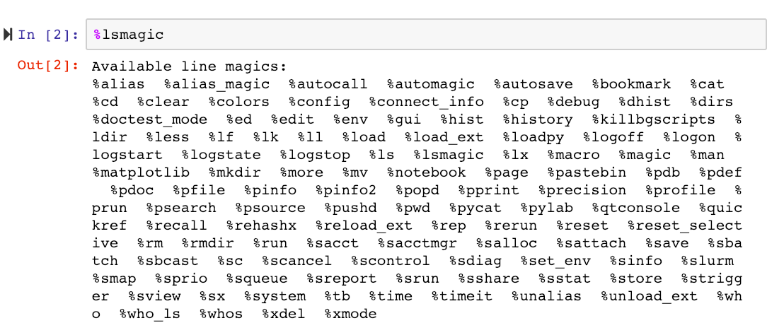
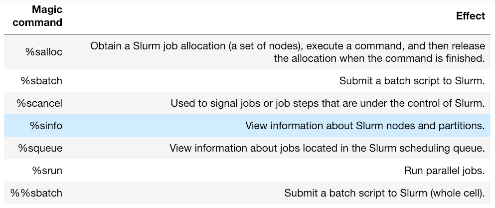
The new SLURM-magics are: %sacct, %sacctmgr, %salloc, %sattach, %sbatch, %sbcast, %scancel, %sdiag, %sinfo, %slurm, %smap, %sprio, %squeue, %sreport, %srun, %sshare, %sstat, %strigger, %sview, %%sbatch.
But only a few of these will be relevant for the majority of researchers using PDC’s facilities.
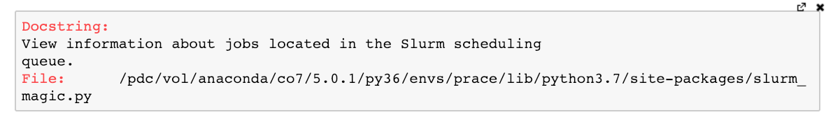
As with any other Jupyter magic command, we can use a question mark to bring up a help menu:

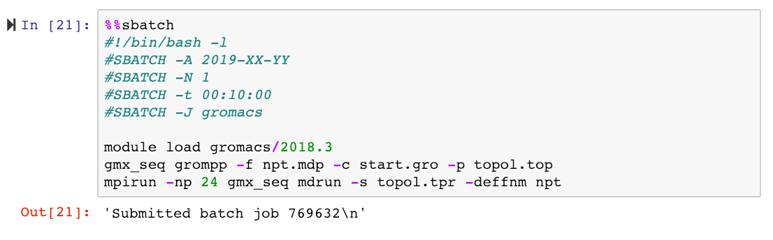
But how do we start batch jobs from within a notebook? By writing our batch script into a code cell and using the %%sbatch cell magic! Cell magics (prepended by %%) differ from line magics (prepended by %) in that the entire cell is affected by the magic. When we execute a cell containing a batch script and the %%sbatch command at the top, the job is submitted to the SLURM queue.
For demonstration purposes we will submit a job which will run a molecular dynamics simulation using the Gromacs package, and we will limit ourselves to Tegner. All the input files needed for this run are provided in this GitHub repository.
Our cell looks like this:
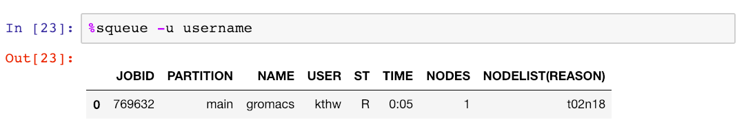
As we are used to doing when working via a regular terminal, we monitor the job using squeue with the -u flag:
Let’s now imagine that we can’t wait for the simulation to finish, and we want to analyse the simulation output on the fly while it’s being generated. This is easily accomplished in the notebook!
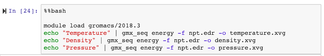
The example HPC application that we’re using, Gromacs, has a utility program which can be used to extract information from the binary output files. To run it, we write shell commands into a code cell containing the %%bash magic to let Jupyter execute a bash script. In our case, we extract time-dependent values of temperature, density and pressure from the simulation:
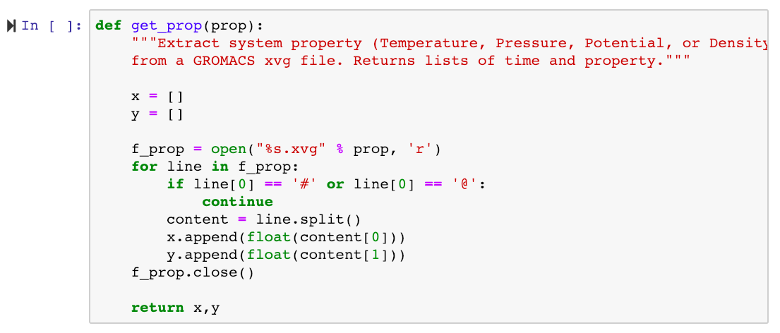
This will create plain text output files (temperature.xvg, density.xvg, pressure.xvg), which we can plot directly in the notebook. But we first write a short function to extract the two columns from an xvg file:
Note that any code run inside our Jupyter session will be executed on the Tegner login node, so we should only run light-weight calculations!
We then import matplotlib, and specify how plots should be displayed in the notebook using the %matplotlib magic:

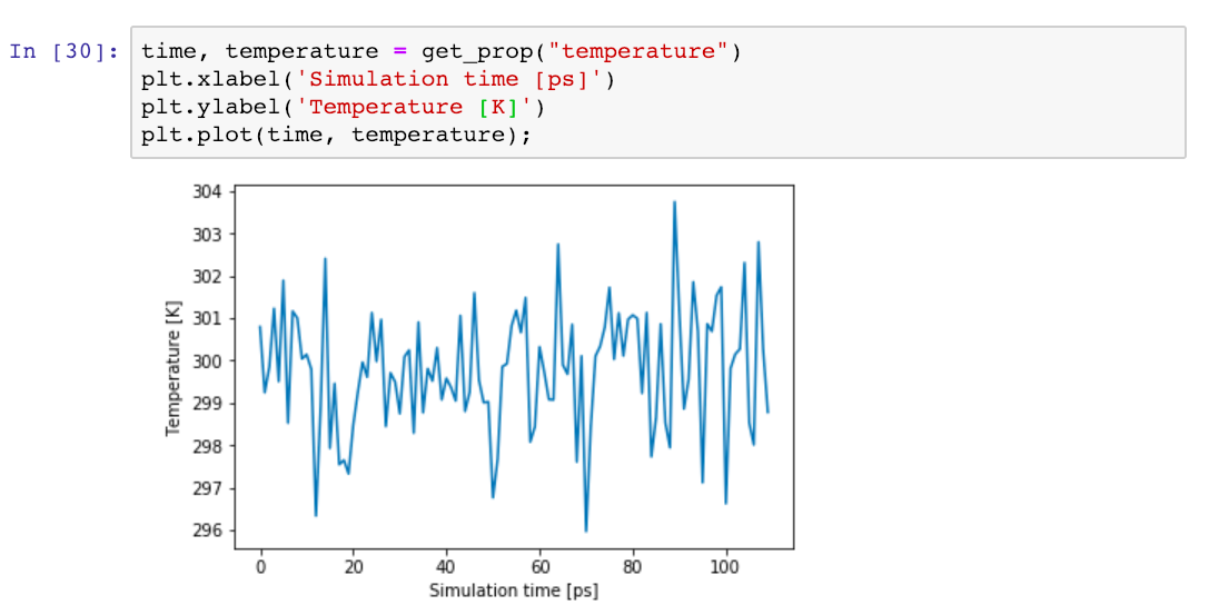
Finally, we can start plotting intermediate results from the running simulation! For example, let’s call our get_prop function for the simulation temperature, and plot the results with added labels to the x- and y-axis:
And that’s it! We could now continue and rerun plotting cells to see how various quantities are evolving with time and visualise other simulation output, but we leave that to the reader. If you want to start from a ready-made notebook containing these steps (and others), you can fetch the 2-slurm-analysis.ipynb notebook from this GitHub repository and open it with Jupyter on Tegner after following the configuration steps and security setup.
Summary
How does the “Jupyter way” compare to the usual approach to pre-processing, running and post-processing jobs? One drawback of the Jupyter way is the overhead involved. The security setup and configuration (config file, password, openssl certificate) only needs to be done once and should be straightforward, but even regular usage requires users to type an extra ssh command to establish the ssh tunnel, copy-paste a URL into the browser, and enter (and remember!) the Jupyter password.
On the other hand, the benefits are that you can start automating your workflows by creating notebooks containing any number of pre-processing steps, batch scripts, monitoring commands and post-processing steps to be performed during and after job execution. This can make HPC workflows more reproducible and shareable, and ready-made notebooks can make it easier, for example, for new PhD students to get started. However, whether Jupyter notebooks suit your HPC work will depend on specifics of the HPC simulation codes and workflows involved, and, ultimately, on whether the user interface of Jupyter appeals to you.